Inspection of the mapping results
Visual inspection of the read alignments in genome browser may be helpful to
- ensure that there is a coverage sufficients for incoming statistics analyses
- re-check the strandness of the library (or check if you did not use the
infer experimenttool) - check contamination by DNA reads (which match intronic sequences)
- produce figures focusing on specific genes you are interested in
- or just because seeing read alignments in a genome is fun and interesting
Bam files are generally the preferred proxies for visualization in genomes browser. However, it is also possible to convert bam files in bigwig format if you are only interested in read coverage, and get this files displayed in genome browsers. Likewise, depending of the genome browser, you may use various file format such as wig, bed, bedgraph, etc.
There are many ways to visualize reads in genome browsers, here we only introduce practically 2 procedures.
The first one is using the remote UCSC genome browser.
The second one is using the local IGV genome browser.
You will see that each procedure has pro and cons.
 UCSC genome browser
The advantage of this genome browser is that it is maintained in a very powerful server which already has numerous annotation tracks for you. In addition, visualisation in UCSC browser is well integrated in Galaxy and transfer of bam information to the remote genome browser is transparent for the Galaxy user. The downside is that your bam alignment must have been produced with UCSC reference genomes, whose chromosomes are, for examples prefixed with "chr", or have different haplotype or contig identifiers from the Genome Resources Consortium (GRC). In some circumstances, you may also find that the UCSC browser is slower than a local genome browser.
As you probably noticed, in our analysis case, we have used the reference GRCm38. The main difference is that the corresponding UCSC mouse genome is mm10 in which chromosomes are prefixed with "chr" (chr1, chr2, chrM, etc.), whereas our GRCm38 reference is not prefixed (1, 2, MT, etc).
In theory it is possible to recode chromosome names in a bam file, but this implies a rather complicated procedure (unpacking the bam in sam, using regex-find-replace tools, repack in bam...)
In practical it is faster (and more reliable) to just realign the reads with a UCSC-compliant mm10 reference !
We are going to do this
- using the
HISAT alignmentshistory → navigate to this history - on the subset of fastqsanger.gz datasets
Dc
 HISAT2 alignments of the Dc fastq.gz datasets.
![]() HISAT2 settings for realignment of the Dc collection
HISAT2 settings for realignment of the Dc collection
-
Source for the reference genome
→ Use a built-in genome
-
Select a reference genome
→ This time select mm10
-
Is this a single or paired library
→ single
-
FASTA/Q file
→ Click first the collection icon
 ,
and select
,
and select 5: DC -
Specify strand information
→ Reverse (R) (we know this now...)
-
Summary Options
→ Output alignment summary in a more machine-friendly style. No
→ Print alignment summary to a file. No (here we don't need these summaries)
-
Leave
Advanced Optionsas is - Press
Execute!
The tool will run during several minutes, generating this time only one dataset collection, which contains the mm10 BAM alignments. As usual take benefit of this run time to rename the collection "Dc BAM alignments to mm10".
If you deploy the collection and its first dataset, you should notice that
- the genome dbkey is now
mm10 - there is a small icon in the form of histogram at the bottom of the dataset.
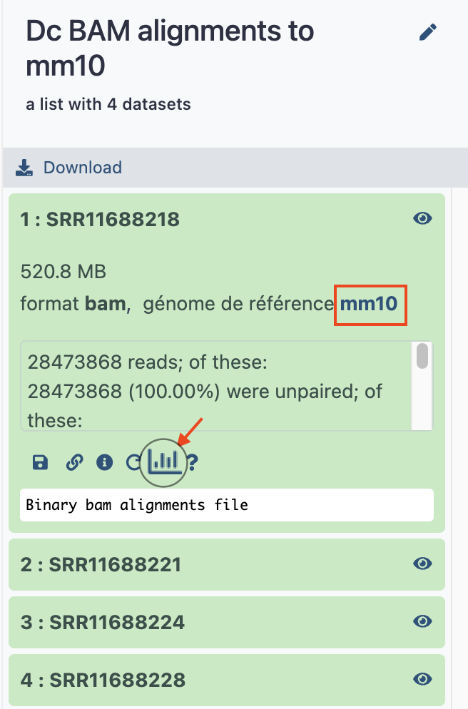
- Click on this icon !
- in the following menu, an option
1. display at UCSC (main , test )is available (it would not be on the bam collection mapped to GRCm38, you may check) - Click on
mainto go to the main UCSC genome browser. - After a few secondes, a new
UCSC Genome Browser on Mouse (GRCm38/mm10)page should directly open - Paste the coordinates
chr15:97,239,883-97,250,884
IGV 
To use IGV with galaxy you need to have this tool on your computer. (If not, you can download IGV from their main site.)
- Open locally IGV
- Click again on the "histogram icon"
-
This time, instead of "display at UCSC (main , test )", click the
locallink in the line2. display with IGV ( local , Mouse mm10 )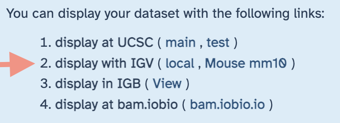
-
 Depending on the size of the bam file you visualise, it can takes several
minutes before data are effectively displayed in the IGV browser.
Depending on the size of the bam file you visualise, it can takes several
minutes before data are effectively displayed in the IGV browser. -
As a last note: IGV has become a powerful local genome browser with integration of remote Galaxy datasets. However the learning curve of IGV is flat at the beginning since it requires a general understanding of network as well as Input/Output mechanisms in Information Technologie. Then, when these issues are mastered, the slope of the IGV LC increase significantly since the Graphical Interface of IGV is in contrast rather intuitive.
 Hang in there, it's definitely worth it !