Markers identification and analyses
We have now grouped our cells according to their transcriptomic profile, we will now have to identify them biologically. If we have enough knowledge of our dataset, we can visualize the expression of the specific genes of the expected populations on the UMAP for example or in Violin Plot in order to determine which cluster will express them the most. It is also possible to identify the specific markers of each cluster by using different expression analyses.
Marker identification
Graphical identification
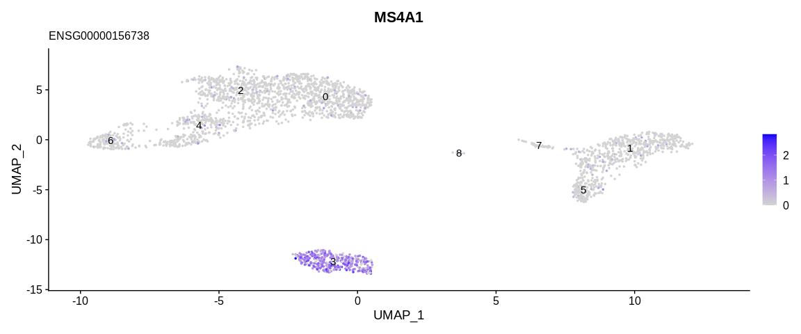
For example, the literature indicates that the MS4A1 gene (associated
with the gene ID ENSG00000156738) is specific to B cells, so by looking
at the expression of this gene on the UMAP or its distribution according
to the clusters thanks to the VlnPlot function we would be able to
determine which cluster would group the B cells.
To do this we will first use the FeaturePlot function which allows us
to visualize our cells on a reduced dimensional space (PCA, UMAP,...) a
continuous variable, it can be the expression of a gene or a continuous
variable of the metadata. Then we will use VlnPlot which allows to
visualize a distribution, by default it will represent a distribution by
cell identity contained in active.ident (we can use the group.by
parameter to use another variable).
FeaturePlot(pbmc_small,                     #SeuratObject
            features = "ENSG00000156738",   #Value to plot, can be a vector of several variable
            reduction = "umap",             #Dimensional reduction to use
            label = TRUE,                   #Plot label on the plot
            label.size = 4) +               #Change label size
  ggtitle(annotated_hg19[annotated_hg19$ensembl_gene_id == "ENSG00000156738", "external_gene_name"],
          "ENSG00000156738")
VlnPlot(pbmc_small,                         #SeuratObject
        features = "ENSG00000156738") +     #Variable to plot
  ggtitle(annotated_hg19[annotated_hg19$ensembl_gene_id == "ENSG00000156738", "external_gene_name"],
          "ENSG00000156738")
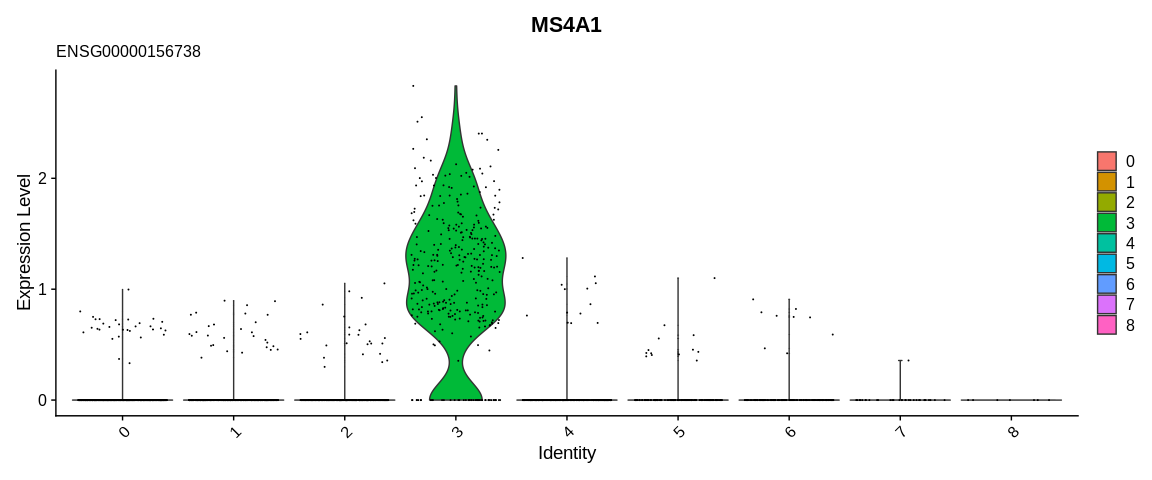
With these results we can consider cluster 3 as being composed of B cells.
Differential expression analysis
It is however sometimes difficult to use this method for each of our clusters. Seurat proposes to identify the specific markers of each cluster using a differential expression analysis method.
For each cluster and each gene, the FindAllMarkers function will determine
if there is a significant difference between the gene expression of the cells
in our cluster and the other cells. By default, it uses the non-parametric
Wilcoxon Rank Sum test (also called Mann-Whitney). He then performs a
Bonferroni multiple correction test.
Here we have changed some parameters to not filter any gene which will be very useful for the enrichment analysis (GSEA) which is based on an ordered list of genes.
pbmc_markers <- FindAllMarkers(pbmc_small,              #SeuratObject
                               only.pos = FALSE,        #Returns positive and negative gene markers
                               min.pct = 0.1,           #Take into account genes that are detected in at least 10% of the cells
                               logfc.threshold = 0,     #Return markers with a logFC superior to threshold
                               test.use = "wilcox",     #Method used
                               verbose = FALSE)

## Preview of the resulting dataframe
kable(head(pbmc_markers))
| p_val | avg_log2FC | pct.1 | pct.2 | p_val_adj | cluster | gene | |
|---|---|---|---|---|---|---|---|
| ENSG00000137154 | 0 | 0.6952948 | 0.998 | 0.997 | 0 | 0 | ENSG00000137154 |
| ENSG00000144713 | 0 | 0.6444963 | 0.998 | 0.997 | 0 | 0 | ENSG00000144713 |
| ENSG00000112306 | 0 | 0.7383383 | 1.000 | 0.994 | 0 | 0 | ENSG00000112306 |
| ENSG00000177954 | 0 | 0.7437027 | 0.998 | 0.994 | 0 | 0 | ENSG00000177954 |
| ENSG00000164587 | 0 | 0.6352699 | 1.000 | 0.997 | 0 | 0 | ENSG00000164587 |
| ENSG00000118181 | 0 | 0.7973422 | 1.000 | 0.978 | 0 | 0 | ENSG00000118181 |
The result of this function is a dataframe with several columns:
p_val: p-value of the statistical test usedavg_log2FC: log2(Fold change +1) between the average expression of the considered cluster and the average expression of the rest of the cellspct.1: percentage of detection of the gene in our clusterpct.2: percentage of detection of the gene in the rest of the cellsp_val_adj: adjusted p-value (Bonferroni correction)cluster: cluster consideredgene: name of the gene
Warning
Be careful not to take into account the names of the lines in this dataframe
for reference. Indeed, it is quite frequent that a gene is defined as a
marker for several clusters which will duplicate the line names and thus
add suffixes in the rows. We would be back to the same problem as if we
were using gene names in Read10X.