Clustering
Clustering
Now that we can observe groups of cells, we need to be able to determine them. For this we will use computational methods of grouping cells, called clustering.
In Seurat, we will use two functions. FindNeighbors allows us to build a
graph of shared nearest neighbors (Shared Nearest Neighbors, SNN). The
nodes represent the cells and the links their proximity in the dimensional
space of the PCA. By default, this function represents only the 20 nearest
neighbors. The links are then removed if there is no proximity reciprocity.
From this SNN graph, FindClusters will determine the clusters by identifying
the most interconnected groups of cells based on the modularity optimization.
This method depends on the resolution we choose. The lower the resolution,
the less clusters there will be.
There is no single valid resolution value, so we will generate the clustering based on several resolution values and determine a posteriori which one best represents our cell populations.
pbmc_small <- FindNeighbors(pbmc_small,          #SeuratObject
                            reduction = "pca",   #Reduction to used
                            k.param = 20,
                            dims = 1:pc_to_keep) #Number of PCs to keep (previously determined)

pbmc_small <- FindClusters(pbmc_small,                                        #SeuratObject
                           resolution = seq(from = 0.2, to = 1.2, by = 0.2),  #Compute clustering with several resolutions (from 0.2 to 1.2 : values usually used)
                           verbose = FALSE)
FindNeighbors builds two graphs available in the object@graphs slot
where we can find all the information about the NN (nearest neighbors)
and SNN (shared nearest neighbors) graphs.
FindClusters adds columns in the metadata with the prefix
[assay]_[graph]_res. followed by the different resolutions computed and
the column seurat_clusters corresponding to the clusters determined in
the last resolution computed. The default cell identity contained in the
active.ident slot has now changed and also corresponds to the cluster
identity of the last computed resolution. Each column will therefore
associate a cluster number for each cell. Cluster numbers are assigned
according to their size (so cluster 0 will always be the one with the
most cells, and so on).
| orig.ident | nCount_RNA | nFeature_RNA | percent_mito | RNA_snn_res.0.2 | RNA_snn_res.0.4 | RNA_snn_res.0.6 | RNA_snn_res.0.8 | RNA_snn_res.1 | RNA_snn_res.1.2 | seurat_clusters | |
|---|---|---|---|---|---|---|---|---|---|---|---|
| AAACATACAACCAC-1 | PBMC analysis | 2421 | 781 | 3.0152829 | 0 | 2 | 2 | 2 | 5 | 5 | 5 |
| AAACATTGAGCTAC-1 | PBMC analysis | 4903 | 1352 | 3.7935958 | 3 | 3 | 3 | 3 | 2 | 2 | 2 |
| AAACATTGATCAGC-1 | PBMC analysis | 3149 | 1131 | 0.8891712 | 0 | 2 | 2 | 2 | 0 | 0 | 0 |
| AAACCGTGCTTCCG-1 | PBMC analysis | 2639 | 960 | 1.7430845 | 1 | 1 | 1 | 1 | 6 | 6 | 6 |
| AAACCGTGTATGCG-1 | PBMC analysis | 981 | 522 | 1.2232416 | 2 | 6 | 6 | 6 | 8 | 8 | 8 |
| AAACGCACTGGTAC-1 | PBMC analysis | 2164 | 782 | 1.6635860 | 0 | 2 | 2 | 2 | 0 | 0 | 0 |
Which resolution to choose?
We have several sets of clusters computed on the basis of different
resolutions. We now have to choose which resolution best represents
our cell populations. The clustree package helps us in this choice.
It represents the relationships and the distribution of the cells within
the clusters at different resolutions.
We use the function of the same name which takes into account seurat
objects, we just need to give it the prefix which will allow us to
retrieve all the resolution columns in our metadata. When this prefix
is removed it must leave only the resolution value for clustree to work.
There are several other parameters to change the aesthetics of the figure
but here we will leave everything as default.
clustree(pbmc_small,               #SeuratObject
         prefix = "RNA_snn_res.")  #Prefix that retrieve all resolution to analyse in cell metadata slot
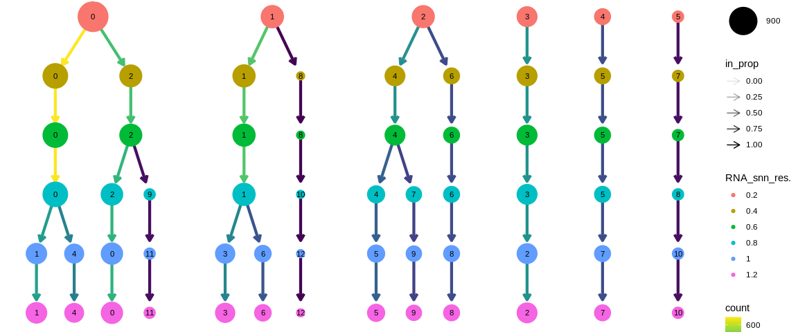
Each point corresponds to a cluster whose size represents the number of cells that compose it and the color, the resolution of the clustering. The first resolution (top) will always be the lowest resolution, then we trace the path of each cell through the clusters of different resolutions (increasingly larger) through the arrows. We analyze here 6 resolutions from 0.2 in red to 1.2 in pink.
The arrows represent the distribution of the clusters of a lower resolution towards the clusters of a higher resolution. For example, the cells of cluster 0 of resolution 0.2 in red are distributed in clusters 0 and 2 of resolution 0.4 in khaki green. While cluster 3 of resolution 0.2 is composed of the same cells as cluster 3 of resolution 0.4. The color of the arrows corresponds to the number of cells of the "parent" cluster which feeds the "child" cluster. The opacity of the arrows represents the proportion of cells coming from the "parent" cluster. It is on this point that clustree allows us to identify the resolution to choose. If a cluster has several origins, then we consider that we have clustered the cells too much and that we should choose a lower resolution.
We can observe the following facts:
- The clustering obtained from the resolutions 0.4 and 0.6 are identical.
- Clusters 3, 4 and 5 from resolution 0.2 are robust until resolution 1.2
Since the clustering results are really clean (no clusters having several origins), it is difficult to determine which resolution to choose without a priori. We can always use the knowledge of our dataset to guide us on the expected number of cell populations. If we don't have any idea, it is better to use a low resolution, to identify the populations with the help of the marker analysis. If this is not conclusive, we can go back to the resolution choice to choose a finer or more general clustering.
Here we will choose the resolution 0.4 or 0.6 because they are identical and therefore with rather robust clusters. We could imagine using the 0.8 to 1.2 clustering to identify sub-populations.
We will update the default identity of the cells that are accessible via
the Idents function. There are several ways to modify the active identity,
either by filling it with a vector composed of the cell identities, or with
the name of a column in our metadata.
## Set the default resolution level
Idents(pbmc_small) <- "RNA_snn_res.0.4"
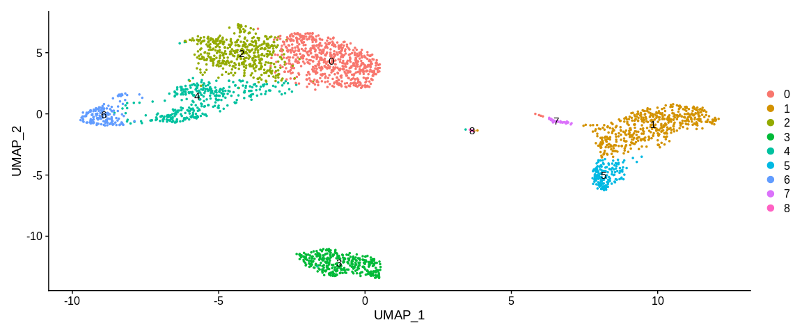
## Visualize clusters in UMAP coordinates
UMAPPlot(pbmc_small, #SeuratObject
label = TRUE, #Plot label on the plot
label.size = 4) #Change label size